
First, using the newly created second inkjet transparency, print another test print using multiple layers according to your times just as before. This is my print of 2-4-8 minutes using my '2-4-8 Neg2 Smooth' curve. This time the highlights have some value to them and the scale extends from zone 1 to zone 9. The scale on the left looks almost perfect if not a little too dark, and the scale on the right is a little darker around zone 9 than it should be, possibly from my uv exposure unit not providing even exposure.
Finally, to complete our custom inkjet negative curve, we have to iron our any kinks with it. The requires at least 1 more test print and averaging the curves for an optimal final curve to be used with all your gum bichromate printing.
A Third Test Print

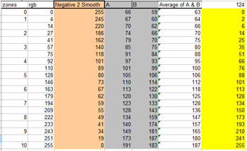
Just as before, record the rbg values your zones become when the second curve is applied (in orange this time). Also enter the mean values of each zone from the 3rd gum print test using your selection tool and histogram pallet as shown earlier. Calculate the average of both the A and B scales in your print, and calculate the relative scale (in yellow).

Enter the input and output values into a new curve. Smooth the curve just as the others with only one click of the smooth button. Save the curve as something like '2-4-8 Neg3 Smooth'

Now if we were to overlay this new curve (lets call it Neg3) with our previous Neg2 curve, we would see that they don't exactly line up. Neg2 printed slightly too dark in gum bichromate, and Neg3 which we have not printed yet should be closer to the right place, but chances are it will print too light. In fact we could continue doing test prints until we go insane, slowly honing in on the perfect curve. But who wants to do that?
Instead we can find an average curve between these two curves that will trace right along the center of them both as shown by the green dashed line.

To find this average curve it would probably take a fair share of complicated math. Fortunately there is an easier way, and we can have photoshop or gimp do the math for us.
First we need to open that original image with the original zone scales that we've been making our transparencies from. We also need to duplicate the layer, in photoshop by hitting ctrl+J and in gimp by pressing Shift+ctrl+D.

Rename each layer by double clicking the label to Neg2 and Neg3
After that apply the Neg2 curve to the Neg2 layer, and similarly, apply the Neg3 curve to the Neg3 Layer

Your images will have inverted according to the curves you applied to them. Now to get that sweet spot between the two curves, change the opacity of the top layer to 50%. Your image is now displaying the average curve. All we have to do is extract the values.

Make another table to hold your numbers. On the left will be the zones and their corresponding rgb values we started with.
Using the eyedropper tool in photoshop we can measure the values of each zone while they are blended together by the 50% opacity. Enter the values in the chart.

Make a final curve, enter the input and output values from the table using the zone rgb values for the inputs, and the output values from the green. The curve should be so smooth that you can save it as is without smoothing it as we have done with our previous curves.
This is it, your final gum bichromate curve! You've survived the days and days of tests! Save it with a good strong name like "FINAL 2-4-8 AVG GUM NEGATIVE CURVE" and use it for all your prints!
Using the Custom Scale
Now that the curve is finished, all that you need to do is open your images and apply the curve before your print any inkjet negatives. You no longer have to use only gray values when you print. If you want to print into the shadows you know you can use your shortest exposure time. Similarly if you want to deepen the highlights with some color you could print with your longest exposure time. There's no reason you have to always print all three of your exposure times.